2024. 7. 6. 21:38ㆍArtificialIntelligence/DeepLearning
Tokenization and Embedding
: Science Behind Large Language Model
Every input that we are providing to GPT is nothing but a token (numerical id) or a sequence of tokens. GPT doesn’t understand the language the way humans do but it just processes sequence of numerical ids, that we call tokens. But how does it find the association among words(tokens) and provide human like response, here comes the concept of embedding?
* 임베딩이란?
- Word embedding is like creating a map for words in vector space. Each word is represented by a unique location on the map, and words with similar meanings are grouped closer together.
(단어 사이의 연관성을 컴퓨터가 이해할 수 있도록) - Word embedding helps the computer understand language better, making it smarter at tasks like translation or answering questions.
- world must be represented in vector space with several hundred dimensions and each word is represented by a distribution of weights across those elements
- Embeddings play a crucial role in enabling machines to grasp the associations and similarities between words
- these embeddings are then fed into Language Models (specifically neural networks) as inputs.
The neural networks churn out another set of tokens based on probability scores.
- The process of how neural networks process these embeddings to generate another set is a topic for another discussion.
- GPT received the bunch of tokens, created it’s embedding, processed it through neural networks and return another set of tokens. (모델이 input으로 들어온 토큰들을 바탕으로, 다른 토큰들(즉 문장)을 생성한다)
- It’s important to note that tokenization is a reversible process. After the model generates output, the tokenizer converts the sequence of token IDs back into human-readable text.
- A helpful rule of thumb is that one token generally corresponds to ~4 characters of text for common English text. This translates to roughly ¾ of a word (so 100 tokens ~= 75 words).
- https://platform.openai.com/tokenizer

The Illustrated Transformer
- The Transformer was proposed in the paper Attention is All You Need
https://sohyeonkim-dev.tistory.com/185
[Paper reading] Attention is all you need, Transformer
Transformer Abstract The dominant sequence transduction models are based on complex recurrent or convolutional neural networks that include an encoder and a decoder. The best performing models also connect the encoder and decoder through an attention mecha
sohyeonkim-dev.tistory.com
- The encoding component is a stack of encoders (the paper stacks six of them on top of each other – there’s nothing magical about the number six, one can definitely experiment with other arrangements).
- The decoding component is a stack of decoders of the same number.
- The encoders are all identical in structure (yet they do not share weights).
Each one is broken down into two sub-layers
: self attention과 Feed-forward Neural Network 2개의 하위 레이어로 구성됨

- The encoder’s inputs first flow through a self-attention layer – a layer that helps the encoder look at other words in the input sentence as it encodes a specific word.
- The outputs of the self-attention layer are fed to a feed-forward neural network.
The exact same feed-forward network is independently applied to each position. - The decoder has both those layers, but between them is an attention layer that helps the decoder focus on relevant parts of the input sentence

* 임베딩 과정
- The embedding only happens in the bottom-most encoder. The abstraction that is common to all the encoders is that they receive a list of vectors each of the size 512 – In the bottom encoder that would be the word embeddings, but in other encoders, it would be the output of the encoder that’s directly below.
- The size of this list is hyperparameter we can set – basically it would be the length of the longest sentence in our training dataset.
- After embedding the words in our input sequence, each of them flows through each of the two layers of the encoder.
- Here we begin to see one key property of the Transformer, which is that the word in each position flows through its own path in the encoder. There are dependencies between these paths in the self-attention layer.
- The feed-forward layer does not have those dependencies, however, and thus the various paths can be executed in parallel while flowing through the feed-forward layer.
- Next, we’ll switch up the example to a shorter sentence and we’ll look at what happens in each sub-layer of the encoder.
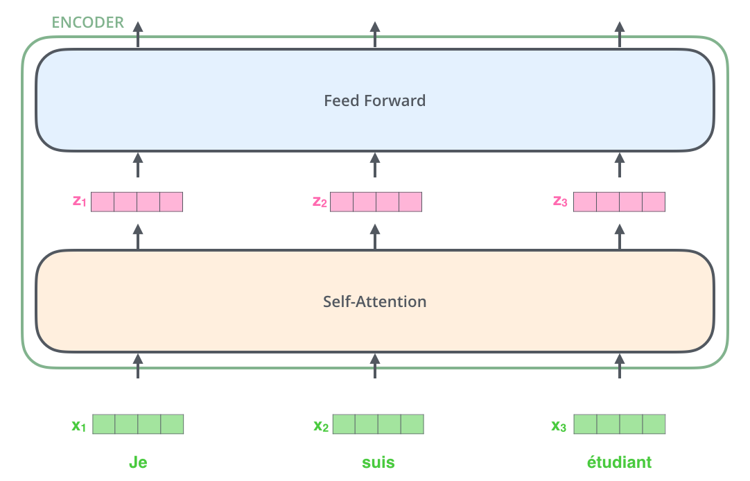

- Encoder receives a list of vectors as input. It processes this list by passing these vectors into a ‘self-attention’ layer, then into a feed-forward neural network, then sends out the output upwards to the next encoder.
- As the model processes each word (each position in the input sequence), self attention allows it to look at other positions in the input sequence for clues that can help lead to a better encoding for this word.
- If you’re familiar with RNNs, think of how maintaining a hidden state allows an RNN to incorporate its representation of previous words/vectors it has processed with the current one it’s processing. Self-attention is the method the Transformer uses to bake the “understanding” of other relevant words into the one we’re currently processing.


* 행렬로 동작 원리 파악하기
- The first step in calculating self-attention is to create three vectors from each of the encoder’s input vectors (in this case, the embedding of each word). So for each word, we create a Query vector, a Key vector, and a Value vector. These vectors are created by multiplying the embedding by three matrices that we trained during the training process.
- Notice that these new vectors are smaller in dimension than the embedding vector. Their dimensionality is 64, while the embedding and encoder input/output vectors have dimensionality of 512. They don’t HAVE to be smaller, this is an architecture choice to make the computation of multiheaded attention (mostly) constant.
* What are the “query”, “key”, and “value” vectors?
- They’re abstractions that are useful for calculating and thinking about attention. Once you proceed with reading how attention is calculated below, you’ll know pretty much all you need to know about the role each of these vectors plays.
- The second step in calculating self-attention is to calculate a score. Say we’re calculating the self-attention for the first word in this example, “Thinking”. We need to score each word of the input sentence against this word. The score determines how much focus to place on other parts of the input sentence as we encode a word at a certain position.
- The score is calculated by taking the dot product of the query vector with the key vector of the respective word we’re scoring. So if we’re processing the self-attention for the word in position #1, the first score would be the dot product of q1 and k1. The second score would be the dot product of q1 and k2.
- The third and fourth steps are to divide the scores by 8 (the square root of the dimension of the key vectors used in the paper – 64. This leads to having more stable gradients. There could be other possible values here, but this is the default), then pass the result through a softmax operation. Softmax normalizes the scores so they’re all positive and add up to 1.
- The fifth step is to multiply each value vector by the softmax score (in preparation to sum them up). The intuition here is to keep intact the values of the word(s) we want to focus on, and drown-out irrelevant words (by multiplying them by tiny numbers like 0.001, for example).
- The sixth step is to sum up the weighted value vectors. This produces the output of the self-attention layer at this position (for the first word).


* Matrix Calculation of Self-Attention
- The first step is to calculate the Query, Key, and Value matrices. We do that by packing our embeddings into a matrix X, and multiplying it by the weight matrices we’ve trained (WQ, WK, WV). Every row in the X matrix corresponds to a word in the input sentence. We again see the difference in size of the embedding vector (512, or 4 boxes in the figure), and the q/k/v vectors (64, or 3 boxes in the figure)
- Finally, since we’re dealing with matrices, we can condense steps two through six in one formula to calculate the outputs of the self-attention layer.
* The Beast With Many Heads
The paper further refined the self-attention layer by adding a mechanism called “multi-headed” attention. (예전에 트랜스포머 논문 읽으면서, 잘 이해되지 않았던 부분.!) This improves the performance of the attention layer in two ways:
- It expands the model’s ability to focus on different positions. Yes, in the example above, z1 contains a little bit of every other encoding, but it could be dominated by the actual word itself. If we’re translating a sentence like “The animal didn’t cross the street because it was too tired”, it would be useful to know which word “it” refers to.
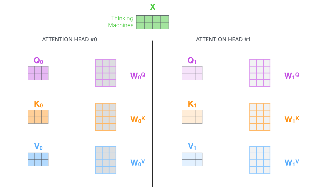
- It gives the attention layer multiple “representation subspaces”. As we’ll see next, with multi-headed attention we have not only one, but multiple sets of Query/Key/Value weight matrices (the Transformer uses eight attention heads, so we end up with eight sets for each encoder/decoder).
Each of these sets is randomly initialized. Then, after training, each set is used to project the input embeddings (or vectors from lower encoders/decoders) into a different representation subspace.
If we do the same self-attention calculation we outlined above, just eight different times with different weight matrices, we end up with eight different Z matrices
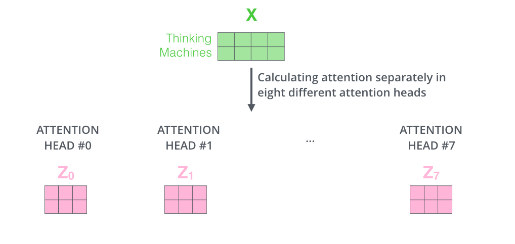

This leaves us with a bit of a challenge. The feed-forward layer is not expecting eight matrices – it’s expecting a single matrix (a vector for each word). So we need a way to condense these eight down into a single matrix.
How do we do that? We concat the matrices then multiply them by an additional weights matrix WO.
That’s pretty much all there is to multi-headed self-attention. It’s quite a handful of matrices, I realize. Let me try to put them all in one visual so we can look at them in one place

Now that we have touched upon attention heads, let’s revisit our example from before to see where the different attention heads are focusing as we encode the word “it” in our example sentence:
If we add all the attention heads to the picture, however, things can be harder to interpret :


* Representing The Order of The Sequence Using Positional Encoding
- One thing that’s missing from the model as we have described it so far is a way to account for the order of the words in the input sequence. (단어들의 순서 정보를 고려하지 않음!)
- To address this, the transformer adds a vector to each input embedding. These vectors follow a specific pattern that the model learns, which helps it determine the position of each word, or the distance between different words in the sequence. The intuition here is that adding these values to the embeddings provides meaningful distances between the embedding vectors once they’re projected into Q/K/V vectors and during dot-product attention. (Positional Encoding 개념)

* What might this pattern look like?
- In the following figure, each row corresponds to a positional encoding of a vector. So the first row would be the vector we’d add to the embedding of the first word in an input sequence. Each row contains 512 values – each with a value between 1 and -1. We’ve color-coded them so the pattern is visible.
- The formula for positional encoding is described in the paper (section 3.5). You can see the code for generating positional encodings in get_timing_signal_1d(). This is not the only possible method for positional encoding. It, however, gives the advantage of being able to scale to unseen lengths of sequences (e.g. if our trained model is asked to translate a sentence longer than any of those in our training set).
- The positional encoding shown above is from the Tensor2Tensor implementation of the Transformer. The method shown in the paper is slightly different in that it doesn’t directly concatenate, but interweaves the two signals.


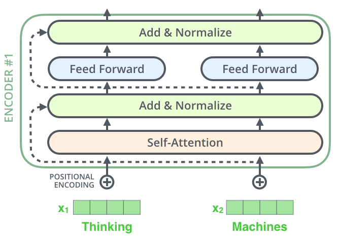
* The Residuals
- One detail in the architecture of the encoder that we need to mention before moving on, is that each sub-layer (self-attention, ffnn) in each encoder has a residual connection around it, and is followed by a layer-normalization step.
- If we’re to visualize the vectors and the layer-norm operation associated with self attention, it would look like this

* The Decoder Side
- Now that we’ve covered most of the concepts on the encoder side, we basically know how the components of decoders work as well. But let’s take a look at how they work together. (조금 다른 점이 있다)
- The encoder start by processing the input sequence. The output of the top encoder is then transformed into a set of attention vectors K and V. These are to be used by each decoder in its “encoder-decoder attention” layer which helps the decoder focus on appropriate places in the input sequence:
- The following steps repeat the process until a special symbol is reached indicating the transformer decoder has completed its output. (모두 출력할 때 까지 반복) The output of each step is fed to the bottom decoder in the next time step, and the decoders bubble up their decoding results just like the encoders did. And just like we did with the encoder inputs, we embed and add positional encoding to those decoder inputs to indicate the position of each word.
- The self attention layers in the decoder operate in a slightly different way than the one in the encoder
- In the decoder, the self-attention layer is only allowed to attend to earlier positions in the output sequence. This is done by masking future positions (setting them to -inf) before the softmax step in the self-attention calculation.
- The “Encoder-Decoder Attention” layer works just like multiheaded self-attention, except it creates its Queries matrix from the layer below it, and takes the Keys and Values matrix from the output of the encoder stack.
* The Final Linear and Softmax Layer
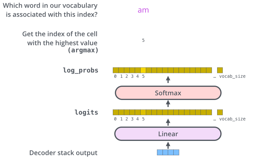
- The decoder stack outputs a vector of floats. How do we turn that into a word? That’s the job of the final Linear layer which is followed by a Softmax Layer.
- The Linear layer is a simple fully connected neural network that projects the vector produced by the stack of decoders, into a much, much larger vector called a logits vector.
- Let’s assume that our model knows 10,000 unique English words (our model’s “output vocabulary”) that it’s learned from its training dataset. This would make the logits vector 10,000 cells wide – each cell corresponding to the score of a unique word. That is how we interpret the output of the model followed by the Linear layer.
- The softmax layer then turns those scores into probabilities (all positive, all add up to 1.0). The cell with the highest probability is chosen, and the word associated with it is produced as the output for this time step.
* Recap Of Training
- Now that we’ve covered the entire forward-pass process through a trained Transformer, it would be useful to glance at the intuition of training the model.
- During training, an untrained model would go through the exact same forward pass. But since we are training it on a labeled training dataset, we can compare its output with the actual correct output.
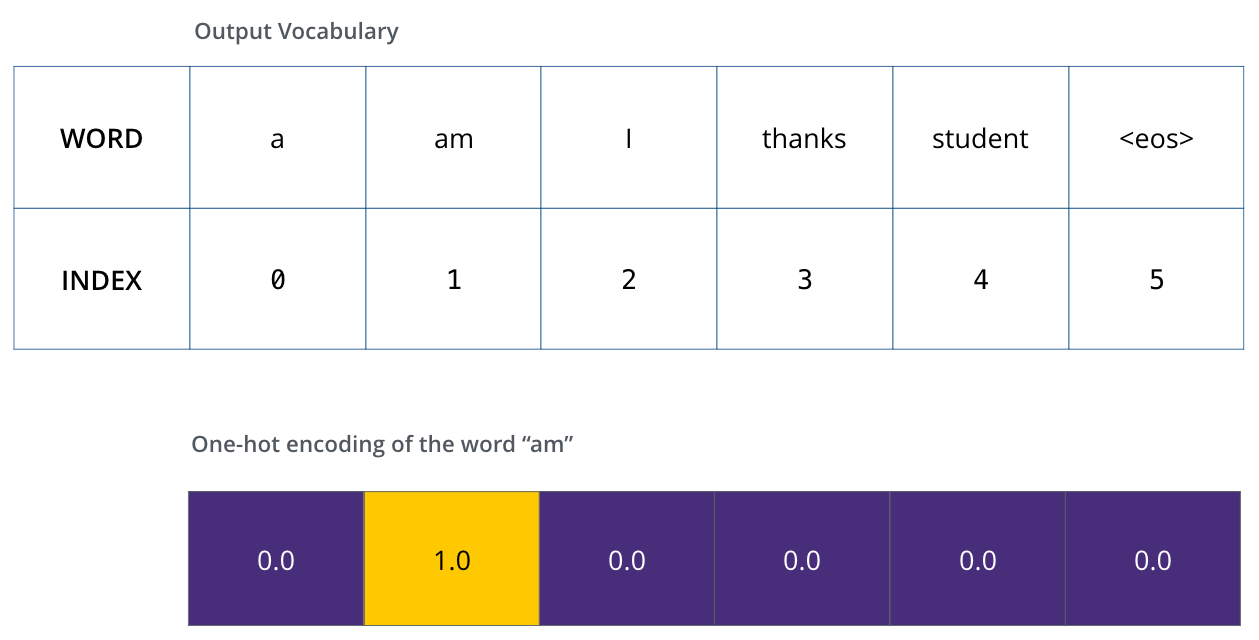
- To visualize this, let’s assume our output vocabulary only contains six words(“a”, “am”, “i”, “thanks”, “student”, and “<eos>” (short for ‘end of sentence’)).
- Once we define our output vocabulary, we can use a vector of the same width to indicate each word in our vocabulary. This also known as one-hot encoding. So for example, we can indicate the word “am” using the following vector
- Following this recap, let’s discuss the model’s loss function – the metric we are optimizing during the training phase to lead up to a trained and hopefully amazingly accurate model.
* The Loss Function
- Say we are training our model. Say it’s our first step in the training phase, and we’re training it on a simple example – translating “merci” into “thanks”.
- What this means, is that we want the output to be a probability distribution indicating the word “thanks”. But since this model is not yet trained, that’s unlikely to happen just yet.
- How do you compare two probability distributions? We simply subtract one from the other. For more details, look at cross-entropy and Kullback–Leibler divergence. (크로스 앤트로비와 KL 다이버전스 개념!)
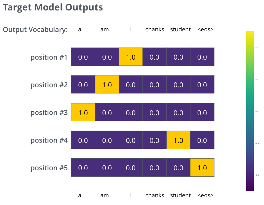
- But note that this is an oversimplified example. More realistically, we’ll use a sentence longer than one word. For example – input: “je suis étudiant” and expected output: “i am a student”. What this really means, is that we want our model to successively output probability distributions where:
- Each probability distribution is represented by a vector of width vocab_size (6 in our toy example, but more realistically a number like 30,000 or 50,000)
- The first probability distribution has the highest probability at the cell associated with the word “i” and the second probability distribution has the highest probability at the cell associated with the word “am”
- And so on, until the fifth output distribution indicates ‘<end of sentence>’ symbol, which also has a cell associated with it from the 10,000 element vocabulary.
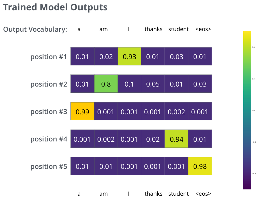
- Now, because the model produces the outputs one at a time, we can assume that the model is selecting the word with the highest probability from that probability distribution and throwing away the rest. That’s one way to do it (called greedy decoding).
- Another way to do it would be to hold on to, say, the top two words (say, ‘I’ and ‘a’ for example), then in the next step, run the model twice: once assuming the first output position was the word ‘I’, and another time assuming the first output position was the word ‘a’, and whichever version produced less error considering both positions #1 and #2 is kept. We repeat this for positions #2 and #3…etc.
- This method is called “beam search”, where in our example, beam_size was two (meaning that at all times, two partial hypotheses (unfinished translations) are kept in memory), and top_beams is also two (meaning we’ll return two translations). These are both hyperparameters that you can experiment with.
LLaMA explained

- Llama is one of the leading state of the art open source large language model released by Meta in 2023
- Llama 1 was originally released with 4 different variants with parameters 6.7B, 13B, 32.5B and 65.2B.
The number of heads in the multi head attention in each of these variants are 32, 40, 52 and 64 respectively as opposed to transformer which had 8 heads in the multi head attention. - each token of the input embedding is represented by a vector of varying dimensions depending on the model size. (기존 트랜스포머 모델이 512를 사용한 것과 달리, 모델 사이즈 별로 다양한 차원의 벡터가 사용됨)
- One of the major change in the llama models as compared to the transformer is the normalization step
- Llama uses a different variant of normalization known as Root Mean Square (RMS) normalization.
- Llama uses rotary positional embedding. This method introduces rotation operations into the positional encoding process allowing the model to learn dynamic positional representations during training rather than relying on pre-calculated static positional encoding vectors.
- Key value (KV) cache is employed in llama to optimize this process where only the key and value vectors are cached while the query vector is updated at each step. This allows the model to reuse the key and value vectors across multiple steps reducing the redundant computations associated with generating each token and thereby making inference faster.
- Grouped multi query attention - while GPUs are quite fast at performing operations on tensors or matrices simply, the bottleneck arises when data needs to be moved around memory and processing units like GPU. So, as memory access increases, the total time complexity of preforming matrix calculations during inference of large language models also increases. (PIM의 문제의식과 동일한 상황.!)
- And, with the addition of KV cache in llama, this problem becomes even more persistent. To solve this multi query attention removes the head (h) dimension from the key (K) and value (V) while keeping it for the Query (Q). This means that all the different query heads will share the same keys and values.
- This results in very faster inference than the usual multi head attention with KV cache with a bit of degradation in quality of output. The grouped multi query attention extends this idea by dividing query into different groups and for each group we have one set of keys and values.
- So, the grouped multi query attention stands in between multi query attention and normal multi head attention maintaining a balanced trade off between speed and quality. (속도와 output의 퀄리티 간 trade-off)
- Another major change in llama from the original transformer is the use of SwiGLU activation function in the feed forward layer instead of the usual ReLU activation. (딥러닝 시간에 교수님이 알려주셨던 swish function!)
- In conclusion, Llama presents a promising advancement in the realm of large language models offering innovative modifications to traditional attention mechanisms such as grouped multi-query attention (더 알아보자), KV caching, RMS normalization and more. It’s open-source nature has sparked a surge in its adoption for fine-tuning across diverse tasks and the introduction of the Llama2 series have also marked a significant advancement delivering even greater performance capabilities.
참고 문헌
GitHub - ggerganov/llama.cpp: LLM inference in C/C++
LLM inference in C/C++. Contribute to ggerganov/llama.cpp development by creating an account on GitHub.
github.com
'ArtificialIntelligence > DeepLearning' 카테고리의 다른 글
| Byte-Pair Encoding tokenization and Tiktoken (0) | 2024.07.08 |
|---|---|
| KSC 2023 학부생 논문 경진대회 우수상 (0) | 2024.02.13 |
| [KSC 2023] KSC 학회 포스터 발표 at BEXCO (0) | 2023.12.22 |
| [GoogleML] Practical Advice for Using ConvNets (0) | 2023.10.07 |
| [Slurm] Dataset Condensation model 돌리기 (feat. 공용GPU) (0) | 2023.09.28 |